-

Bernie Sanders on the U.S. health care system
At Harvard Chan School event, the senator from Vermont calls system “totally broken”Read more -
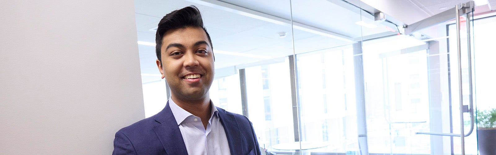
Researching new ways to prevent Alzheimer’s
For Irfan Chaudhuri, SM ’24, his grandparents’ lives helped inspire his path to public health and neuropsychiatric epidemiologyRead more -
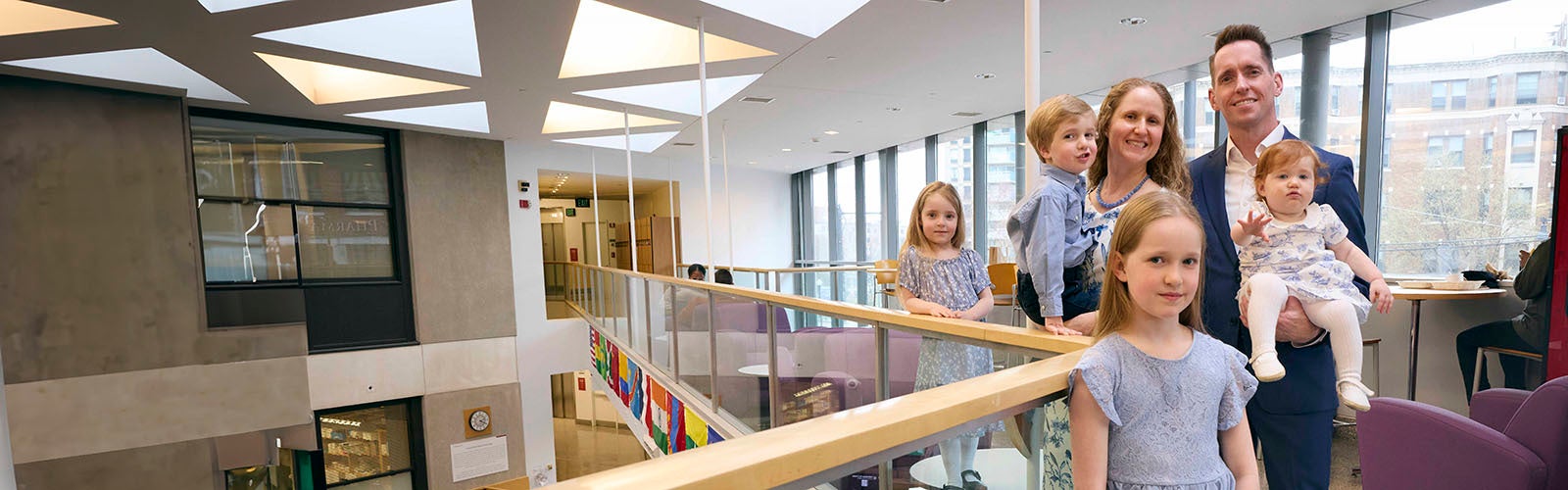
Studying by day, changing diapers by night
Matt and Sally Hamm met in the Air Force, got married, worked as flight surgeons, had four kids, and will soon finish Harvard Chan’s Occupational and Environmental Medicine Residency ProgramRead more -

Measles outbreaks and under-vaccination
Infectious disease expert Yonatan Grad discusses the resurgence of the highly transmissible, preventable diseaseRead more -
When women give birth while in prison, how do their children fare?
Research by Bethany Kotlar, PhD ’24, follows children born to incarcerated mothers for the first three years of their livesRead more